Blog posts with rmarkdown on Jekyll with servr and knitr
So I’m trying to set up my jekyll system to allow me to edit rmarkdown files and insert them into the jekyll system.
This is one way, but I couldn’t get this to work (too impatient), and in the end I found this post with a neat script which I have edited. My edits are mainly to fix the issue that my jekyll instance runs in a /blog/ subdirectory, and also to allow rebuilding of a page by removing the previously generated ../fig/xxx directory from a previous run of the script. I’m sure that there will be easier ways to accomplish this (without the hard coding of the /blog) but I’m too much of a novice with jekyll.
#!/usr/bin/env Rscript

input <- commandArgs(trailingOnly = TRUE)
#KnitPost <- function(input, base.url = "/") {
KnitPost <- function(input, base.url = "/blog/") {
    require(knitr)
    opts_knit$set(base.url = base.url)
# fig.path <- paste0("../figs/", sub(".Rmd$", "", basename(input)), "/")
    fig.path <- paste0("figs/", sub(".Rmd$", "", basename(input)), "/")
    opts_chunk$set(fig.path = fig.path)
    opts_chunk$set(fig.cap = "center")
    render_jekyll()
    print(paste0("../_posts/", sub(".Rmd$", "", basename(input)), ".mkd"))
    knit(input, output = paste0("../_posts/", sub(".Rmd$", "", basename(input)), ".mkd"), envir = parent.frame())
# now move the fig file
# 1 but remove existing directory first
    rm.command<-paste0("rm -r ","../figs/", sub(".Rmd$", "", basename(input)), "/")
# 2 - create a system command to move from the subdir to the parent directory,
    mv.command<-paste0("mv ","figs/", sub(".Rmd$", "", basename(input)), "/", " ../figs/")
# 3 - now run it
    system(rm.command)
    system(mv.command)
}

KnitPost(input)
So let’s try some R…
install.packages(c('servr', 'knitr'), repos = 'http://cran.rstudio.com')R code chunks
Following is from here
Now we write some R code chunks in this post. For example,
options(digits = 3)
cat("hello world!")
## hello world!set.seed(123)
(x = rnorm(40) + 10)## [1] 9.44 9.77 11.56 10.07 10.13 11.72 10.46 8.73 9.31 9.55 11.22
## [12] 10.36 10.40 10.11 9.44 11.79 10.50 8.03 10.70 9.53 8.93 9.78
## [23] 8.97 9.27 9.37 8.31 10.84 10.15 8.86 11.25 10.43 9.70 10.90
## [34] 10.88 10.82 10.69 10.55 9.94 9.69 9.62# generate a table
knitr::kable(head(mtcars))| mpg | cyl | disp | hp | drat | wt | qsec | vs | am | gear | carb | |
|---|---|---|---|---|---|---|---|---|---|---|---|
| Mazda RX4 | 21.0 | 6 | 160 | 110 | 3.90 | 2.62 | 16.5 | 0 | 1 | 4 | 4 |
| Mazda RX4 Wag | 21.0 | 6 | 160 | 110 | 3.90 | 2.88 | 17.0 | 0 | 1 | 4 | 4 |
| Datsun 710 | 22.8 | 4 | 108 | 93 | 3.85 | 2.32 | 18.6 | 1 | 1 | 4 | 1 |
| Hornet 4 Drive | 21.4 | 6 | 258 | 110 | 3.08 | 3.21 | 19.4 | 1 | 0 | 3 | 1 |
| Hornet Sportabout | 18.7 | 8 | 360 | 175 | 3.15 | 3.44 | 17.0 | 0 | 0 | 3 | 2 |
| Valiant | 18.1 | 6 | 225 | 105 | 2.76 | 3.46 | 20.2 | 1 | 0 | 3 | 1 |
(function() {
  if (TRUE) 1 + 1  # a boring comment
})()
## [1] 2names(formals(servr::jekyll)) # arguments of the jekyll() function## [1] "dir" "input" "output" "script" "serve" "command" "..."Just to test inline R expressions1 in knitr, we know the first element in x (created in the code chunk above) is 9.44. You can certainly draw some graphs as well:
par(mar = c(4, 4, .1, .1))
plot(cars, pch = 19, col = 'red')  # a scatterplot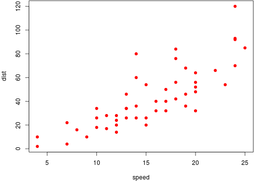
Other ways to do this
* http://rmarkdown.rstudio.com/rmarkdown_websites.html
-
The syntax in R Markdown for inline expressions is
` r code`, wherecodeis the R expression that you want to evaluate, e.g.x[1]. ↩
Leave a Comment